How to sample points from nonrectangular domains?

Recall the previous circle problem. We needed a square that enclosed the circle. Which of the two situations will be more efficient?

Clearly the case on the right is better. We will have fewer wasted darts in the smaller blue square area on the right.
Similarly, the case on the right in the figure below will be more accurate.
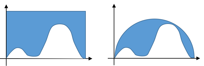
But how do we sample uniformly under the half circle the right figure?
- For a rectangle, we just used a uniform random number generator to get random x and y points.
- There are routines for generating random points that fit some given distribution, such as normally distributed random points.

Approach

Let the curve we want to generate points on be $g(x)$.
Let $G(x)=\int_a^xg(x)dx,$ where $a$ is the lower bound of integration.
We sample uniformly on $G$ and invert to find the corresponding $x=G^{-1}$.
The resulting $x$ locations will be distributed consistent with $g(x)$.
To get the $y$ location of a point corresponding to $x$, we sample a random number uniformly on $[0,\,g(x)]$.

import numpy as np
import matplotlib.pyplot as plt
%matplotlib inline
from scipy.special import erf
from scipy.optimize import fsolve
from scipy.integrate import quad

plt.rc('font', size=14)

def make_plot():

    μ = 2
    σ = 0.5
    x = np.linspace(0,4,100)
    g = 1/np.sqrt(2*np.pi*σ**2)*np.exp(-1/2/σ**2*(x-μ)**2)
    G = 0.5*(1+erf(1/σ/np.sqrt(2)*(x-μ))) 
    
    fig, (ax1, ax2) = plt.subplots(1,2, figsize=(10,5))
    ax1.plot(x,g)
    ax1.set_xlabel('x'); ax1.set_ylabel('g(x)')
    ax1.set_xlim([0,4]); ax1.set_ylim([-0.1,1])
    ax2.plot(x,G)
    ax2.set_xlabel('x'); ax2.set_ylabel('G(x)')
    ax2.set_xlim([0,4]); ax2.set_ylim([-0.1,1])
    
    def Ginv(xFind, Gwant):
        return 0.5*(1+erf(1/σ/np.sqrt(2)*(xFind-μ))) - Gwant
    for yy in np.linspace(0.01,0.99,15):
        xx = fsolve(Ginv, μ, args=yy)[0]
        ax2.arrow(4, yy, xx-4+0.1, 0,      head_width=0.02, head_length=0.1,  fc='gray', ec='gray', linestyle='dashed')
        ax2.arrow(xx, yy, 0, -yy+0.05-0.1, head_width=0.05, head_length=0.05, fc='gray', ec='gray')
    
    plt.tight_layout()

make_plot()

Example: let $g(x)$ be a normal distribution

n    = 2000                        # number of points

#---------- Define g(x)

μ    = 2                           
σ    = 0.5
maxG = 1.0
def g(x):
    return 1/np.sqrt(2*np.pi*σ**2)*np.exp(-1/2/σ**2*(x-μ)**2)

#---------- get g(x) distributed random x points

rG = np.random.rand(n)*maxG      # uniform samples on G
rx = np.empty(n)                 # corresponding x locations found next

def Ginv(xFind, Ggiven):          # inverse function: G --> x
    return 0.5*(1+erf(1/σ/np.sqrt(2)*(xFind-μ))) - Ggiven
for i, rGi in enumerate(rG):
    rx[i] = fsolve(Ginv, μ, args=rGi)
    
#---------- get y points below g(x)
    
ry = np.empty(n)
for i in range(n):
    ry[i] = np.random.rand()*g(rx[i])

#---------- plot results

/var/folders/_7/42qnnz6j17g26jhlhv2l5_580000gn/T/ipykernel_55618/596636519.py:19: DeprecationWarning: Conversion of an array with ndim > 0 to a scalar is deprecated, and will error in future. Ensure you extract a single element from your array before performing this operation. (Deprecated NumPy 1.25.)
  rx[i] = fsolve(Ginv, μ, args=rGi)

x = np.linspace(0,2*μ,100)

fig,ax = plt.subplots(figsize=(10,5))
ax.plot(x,g(x), 'k-');
ax.plot(rx, ry, 'b.', markersize=2);
ax.plot(rx, np.random.rand(len(rx))*0.04-0.02-0.04, '.', markersize=1.0, color='red')
ax.set_xlabel('x');
ax.set_ylabel('g(x)');

Sampling nonuniformly distributed random numbers

Most random number generators provide uniformly distributed random numbers on the domain $[0,\,1]$.
In the previous example, we saw how to sample random points that are normally distributed.
- Specifically, the selection of $x$ points will be normally distributed.
- This means that there are more $x$ points near $\mu$ where the peak is, than on the tails.
- In the above example, we also found corresponding random $y$ points.
- However, in this section, we are only interested in the nonuniformly distributed $x$ points.
- For example, plotting a histogram of the rx points above gives:

plt.hist(rx, 40, rwidth=0.8);

The previous method is difficult if the integration of $g(x)$ is complex or expensive and/or if the subsequent inversion of $G(x)$ is complex or expensive.
Another method for sampling uniformly distributed points from a nonrectangular region is similar to the MC integration problem.
However, we are not doing integration here, only showing another method for sampling from a nonuniform distribution.
This method does not require integration of $g(x)$ or inversion of $G(x)$.
We draw a bounding curve $F(x)$ that is easy to integrate and invert. This could be a rectangle.
- $F(x)$ is everywhere greater than $g(x)$.
Then we draw an $r_x$ point from from the bounding curve, as previously described (using G(x)).
Now we accept the sample point with probability $g(r_x)/F(r_x)$.
- This is done by sampling a random number between 0 and 1. If the random number is less than $g(r_x)/F(r_x)$, then we accept the point, otherwise we reject it.
This approach is called the rejection method.

Example

Sample random normally distributed variables using the rejection method.

def make_plot2():
    n    = 8000                 # random numbers to try (not all kept)
    μ    = 2                           
    σ    = 0.5
    def g(x):
        return 1/np.sqrt(2*np.pi*σ**2)*np.exp(-1/2/σ**2*(x-μ)**2)
    def F(x):                   # bounding function, here a simple uniform profile
        return 1
    
    #-----------------
    
    nkeep = 0                   # total number kept: incremented below
    rx_all = np.empty(0)        # storage for all points: expanded below
    
    for i in range(n):
        rx = np.random.rand()*2*μ
        Paccept = g(rx)/F(rx)
        r  = np.random.rand()        
        if r<Paccept:
            rx_all=np.append(rx_all, rx)
            nkeep += 1
            
    #-----------------
    
    plt.hist(rx_all, 40, rwidth=0.8);
    plt.xlim([0,4])

make_plot2()

Example-Poisson Process

Poisson Processes are extremely important in probability theory.
Used to model random processes in time and space
- Raindrop spacing, radioactive decay, eddies in turbulence, etc.

Raindrops

Suppose it’s raining and you listen to the time spacing of droplets.
There will be some average rate.
But sometimes droplets will be very close together, and sometimes far apart.

Question: what is the distribution of the spacing between events; and can we model this?

Find the PDF of intervals between events; that is $p(\Delta t_e)$.
Assume events occur randomly in time with a mean event rate $\lambda$ (=) $s^{-1}$. That is, $\lambda$ drops per second, on average.
Assume events are statistically independent of each other.
The probability of getting an event in some interval $dt$ is $\lambda dt$, or $dt/T$, where $T=1/\lambda$ is the mean time between events.
Consider the interval $(t_0,\,t_0+\Delta t_e)$, with some sub-intervals:

|  1     2     3     4  |
|-----|-----|-----|-----|
| dt    dt    dt    dt  |

$\phantom{xxx}t_0\phantom{xxxxxxxxxxxxxxxxxx}t_0+\Delta t_e$

The probability of not getting an event in sub-interval 1 is $1-\lambda dt$.
The probability of not getting an event in sub-interval 1 and sub-interval 2 and $\ldots$ sub-interval 4 is

$$(1-\lambda dt)^4,$$

or, for $n$ sub-intervals

$$(1-\lambda dt)^n \rightarrow (1-\lambda dt)^{\Delta t_e/dt}$$

Now, let $dt\rightarrow 0$.
$P(t_{\text{next event}}>\Delta t_e) = \lim_{dt\rightarrow 0}(1-\lambda dt)^{\Delta t_e/dt}$.
Now, at $dt=0$ we have $1^{\infty}$. Work on this:
Now, at $dt=0$ we have $0/0$, so use L’Hopital’s Rule.

$$\ln P = \lim_{dt\rightarrow 0}\frac{-\lambda \Delta t_e}{(1-\lambda dt)} = -\lambda \Delta t_e.$$

Hence,

$$P(t_{\text{next event}}>\Delta t_e) = e^{-\lambda \Delta t_e}.$$

Or,

$$P(t_{\text{next event}}<\Delta t_e) = 1- e^{-\lambda \Delta t_e}.$$

This is a cumulative distribution function.
Differentiate it to get the probability density function:

$$p(\Delta t_e) = \lambda e^{-\lambda \Delta t_e}.$$

This is an exponential distribution.
So, to generate exponentially-distributed events, randomly sample $\Delta t_e$ values from this distribution.
- As above, draw uniform samples of $P(\Delta t_e)$ (the cumulative distribution function) on $[0,\,1]$. Invert this function to get $\Delta t_e$.
- The inversion, is just solving the expression for $P(\Delta t_e)$ for $\Delta t_e$, where $P$ values are taken as random numbers between 0 and 1:
$$\Delta t_e = -\frac{\ln(1-P)}{\lambda}.$$

def make_plot3():
    λ = 1                   
    n = 2000
    rP = np.random.rand(n)
    Δt_e = -np.log(1-rP)/λ
    
    x = np.linspace(0,8,1000)
    y = λ*np.exp(-λ*x)
    
    times = np.cumsum(Δt_e[:40])
    
    plt.rc('font', size=14);
    fig,(ax1,ax2) = plt.subplots(1,2,figsize=(10,5))
    
    ax1.hist(Δt_e, 80, density=True, rwidth=0.8);
    ax1.plot(x,y, linewidth=3);
    ax1.set_xlabel(r'$\Delta t_e$');
    ax1.set_ylabel(r'$p(\Delta t_e)$');
    ax1.set_xlim([0,5])
    
    ax2.plot(times, np.zeros(len(times)), '.', markersize=5)
    for t in times:
        ax2.axvline(x=t, ymin=0.45, ymax=0.55, linewidth=1, color='gray')
    ax2.set_xlabel('time')
    ax2.set_ylim([-1,1])
    
    plt.tight_layout()

make_plot3()