Parabolic PDEs

Outline

FTCS: Forward time centered space
BTCS: Backward time centered space
CN: Crank Nicolson
MOL: Method of lines

Setup

The PDE we’ll consider here is the unsteady diffusion equation.
$$\frac{\partial f}{\partial t} = \alpha\frac{\partial^2f}{\partial x^2}.$$
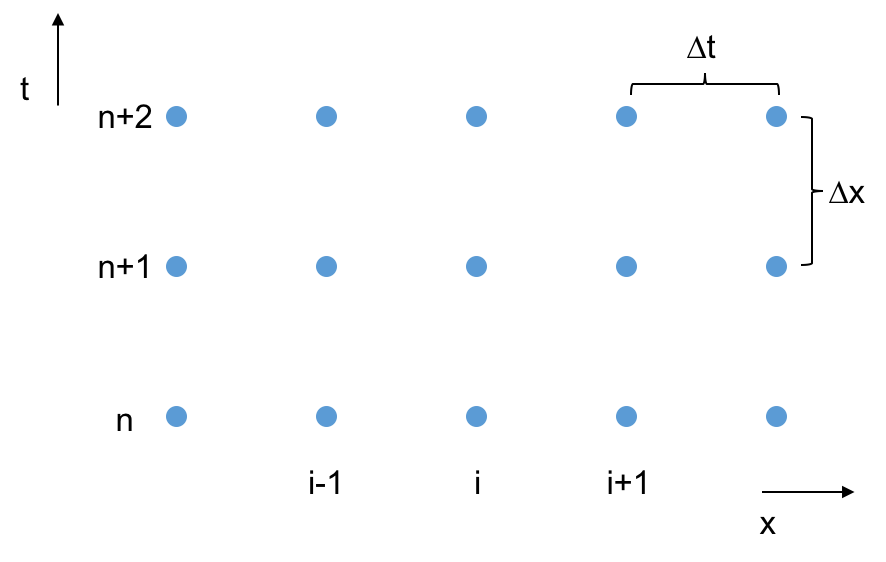
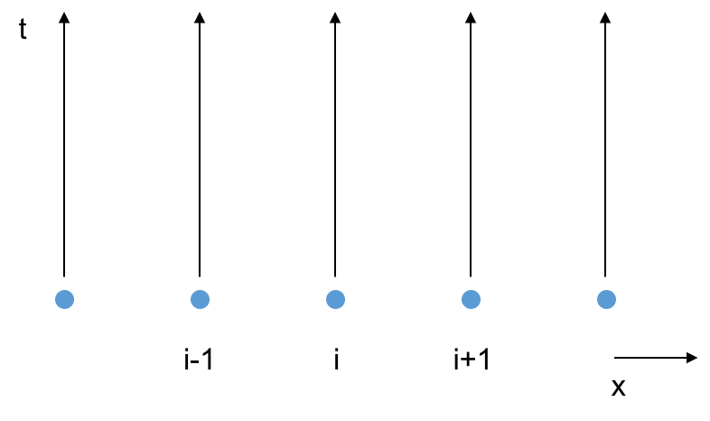
The grid:

FTCS

Forward difference approximation for the time derivative.
Central difference approximation for the space derivative.
Evaluate the spatial term at the old time.
- This is like Explicit Euler at point $n$ in time.
Explicit
First order in time
Second order in space

$$\frac{\partial f}{\partial t} = \alpha\frac{\partial^2f}{\partial x^2},$$$$\frac{f_i^{n+1}-f_i^n}{\Delta t} = \alpha\frac{f_{i-1}^n - 2f_i^n + f_{i+1}^n}{\Delta x^2},$$$$f_i^{n+1}=f_i^n + \frac{\alpha\Delta t}{\Delta x^2}(f_{i-1}^n - 2f_i^n + f_{i+1}^n).$$ $$f_i^{n+1}=f_i^n + d\cdot(f_{i-1}^n - 2f_i^n + f_{i+1}^n),$$ $$d = \frac{\alpha\Delta t}{\Delta x^2}.$$

Approach

Start with the initial condition
Advance each grid point in time based on itself and its neighbors at the previous time.
BC’s are as for boundary value problems.

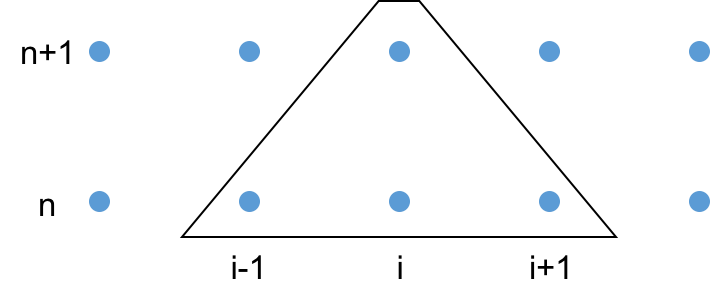
Stencil

BTCS

Backward difference approximation for the time derivative.
Central difference approximation for the space derivative.
Evaluate the spatial term at the new time.
- This is like Implicit Euler at point $n+1$ in time.
Implicit
First order in time
Second order in space

$$\frac{\partial f}{\partial t} = \alpha\frac{\partial^2f}{\partial x^2},$$$$\frac{f_i^{n+1}-f_i^n}{\Delta t} = \alpha\frac{f_{i-1}^{n+1} - 2f_i^{n+1} + f_{i+1}^{n+1}}{\Delta x^2},$$$$f_{i-1}^{n+1} - \left(2+\frac{\Delta x^2}{\alpha\Delta t}\right)f_i^{n+1} + f_{i+1}^{n+1} = -\frac{\Delta x^2}{\alpha\Delta t}f_i^n.$$$$f_{i-1}^{n+1} - \left(2+\frac{1}{d}\right)f_i^{n+1} + f_{i+1}^{n+1} = -\frac{1}{d}f_i^n.$$ $$l_if_{i-1}^{n+1} + a_if_i^{n+1} + u_if_{i+1}^{n+1} = b_i,$$ $$l_i = 1,$$ $$a_i = -\left(2+\frac{1}{d}\right),$$ $$u_i = 1,$$ $$b_i = -\frac{1}{d}f_i^n.$$

Approach

Start with the initial condition.
Advance in time by solving a coupled tridiagonal system of equations at each timestep.
BC’s are as for boundary value problems.

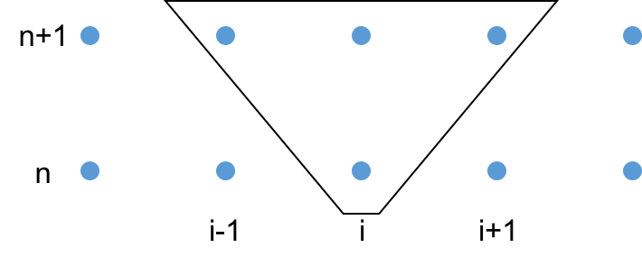
Stencil

Crank Nicolson (CN)

Do 50/50 FTCS and BTCS
This is like the Implicit Trapazoid Method for initial value problems.
This results in a linear tridiagonal system of equations at each timestep, as for the BTCS method, but with slightly different coefficients and a different $b$ vector (right hand side).

$$\frac{\partial f}{\partial t} = \alpha\frac{\partial^2f}{\partial x^2},$$$$\frac{f_i^{n+1}-f_i^n}{\Delta t} = \frac{\alpha}{\Delta x^2}\frac{(f_{i-1}^n - 2f_i^n + f_{i+1}^n)+(f_{i-1}^{n+1} - 2f_i^{n+1} + f_{i+1}^{n+1})}{2},$$$$\left(\frac{d}{2}\right)f_{i-1}^{n+1} -(d+1)f_i^{n+1} + \left(\frac{d}{2}\right)f_{i+1}^{n+1}= -\left(\frac{d}{2}\right)f_{i-1}^n +(d-1)f_i^n - \left(\frac{d}{2}\right)f_{i+1}^n,$$$$f_{i-1}^{n+1} - 2\left(1+\frac{1}{d}\right)f_i^{n+1} + f_{i+1}^{n+1} = -f_{i-1}^n + 2\left(1-\frac{1}{d}\right)f_i^n - f_{i+1}^n.$$ $$l_if_{i-1}^{n+1} + a_if_i^{n+1} + u_if_{i+1}^{n+1} = b_i,$$ $$l_i = 1,$$ $$a_i = -2\left(1+\frac{1}{d}\right),$$ $$u_i = 1,$$ $$b_i = -f_{i-1}^n + 2\left(1-\frac{1}{d}\right)f_i^n - f_{i+1}^n.$$

Implicit
Second order in time
Second order in space

Approach

Start with the initial condition.
Advance in time by solving a coupled tridiagonal system of equations at each timestep.
BC’s are as for boundary value problems.

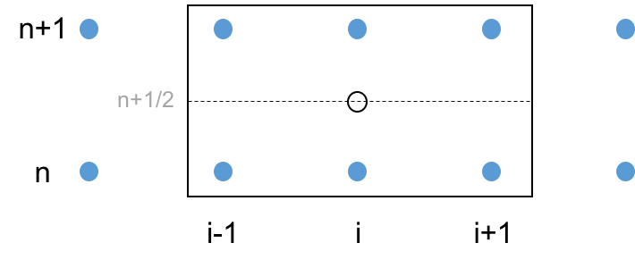
Stencil

Derivation

This method can be derived by writing two Taylor series about a fictional grid point at $(n+\frac{1}{2},\, i)$, evaluated at point $n$, and point $n+1$.

$$ f_i^n = f_i^{n+1/2} - \frac{\Delta t}{2}\left.\frac{\partial f}{\partial t}\right|^{n+1/2}_i + \frac{\Delta t^2}{4}\left.\frac{\partial^2f}{\partial t^2}\right|_i^{n+1/2} + \mathcal{O}(\Delta t^3),$$$$ f_i^{n+1} = f_i^{n+1/2} + \frac{\Delta t}{2}\left.\frac{\partial f}{\partial t}\right|^{n+1/2}_i + \frac{\Delta t^2}{4}\left.\frac{\partial^2f}{\partial t^2}\right|_i^{n+1/2} + \mathcal{O}(\Delta t^3),$$

Subtract the first equation from the second:

$$ f_i^{n+1} - f_i^n = \Delta t\left.\frac{\partial f}{\partial t}\right|_i^{n+1/2} + \mathcal{O}(\Delta t^3).$$

Now, we take

$$\left.\frac{\partial f}{\partial t}\right|_i^{n+1/2} = \frac{1}{2}\left(\left.\frac{\partial f}{\partial t}\right|_i^n + \left.\frac{\partial f}{\partial t}\right|_i^{n+1}\right) = \frac{1}{2}\frac{\alpha}{\Delta x^2}[(f_{i-1}^n - 2f_i^n + f_{i+1}^n)+(f_{i-1}^{n+1} - 2f_i^{n+1} + f_{i+1}^{n+1})].$$

Inserting gives

$$f_i^{n+1} - f_i^n = \frac{\Delta t}{2}\frac{\alpha}{\Delta x^2}[(f_{i-1}^n - 2f_i^n + f_{i+1}^n)+(f_{i-1}^{n+1} - 2f_i^{n+1} + f_{i+1}^{n+1})],$$

which rearranges to the final result.

Generalization

The CN method can be generalized to an $\omega$ method.
Instead of taking a 50/50 split of the RHS at old and new times, we can take some other combination:

$$\frac{f_i^{n+1}-f_i^n}{\Delta t} = \alpha\left[\omega\left(\frac{\partial^2f}{\partial x^2}\right)_i^{n+1} + (1-\omega)\left(\frac{\partial^2f}{\partial x^2}\right)_i^n\right].$$

For $\omega=0$ we have FTCS.
For $\omega=1$ we have BTCS.
For $\omega=1/2$ we have CN.

Method of Lines (MOL)

Discretize just the spatial domain, but not the time domain.

$$\frac{\partial f_i}{\partial t} = \frac{\alpha}{\Delta x^2}(f_{i-1} - 2f_i + f_{i+1}).$$

This is now a coupled system of ODEs.
- We have one ODE for each grid point $i$.
The is formulated as continuous in time, and discrete in space.

Normally, the ODE solver will also discretize in time, but this is done internally.
- (we still end up with a discrete solution in time and space).
- time domain might not have uniform grid spacing, as per the ODE solver chosen.