Tree Structure

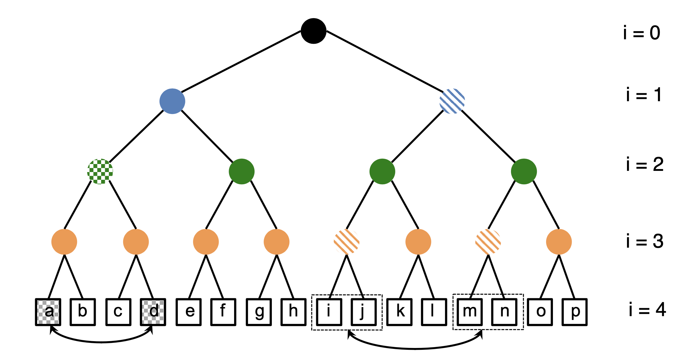
In the following, a summary of the model is provided. A more detailed version can be found in [1]. The structure is based on a binary tree consisting of a hierarchy of nodes (represented by circles). At the base (bottom) of the tree, there are fluid parcels (represented by squares). The tree has five levels (indexed from 0 to 4). The top node, or apex, divides into two subtrees, each starting from a node one level below. Each of these nodes divides further into smaller subtrees. This pattern continues down to the base, where fluid properties are stored in parcels, and additional length and time scale information is associated with the nodes at each level.

For an N-level binary tree, the number of fluid parcels is $2^{N-1}$, and the length scale at each level is reduced by a factor of $A$ from the previous level, given by $L_{i+1} = L_iA$, which can be expressed as:

$$ L_i = L_0A^{i} $$

where $A < 1$. This shows the multiplicative reduction in length scales as the tree progresses downward. In this model, the volume of each subtree is half that of its parent level. For three-dimensional space, we set $A = 1/2^{1/3}$, which maintains the volume halving along with the corresponding length scale reduction. In the general case, with $D$ dimensions, $A$ is calculated as $1/2^{1/D}$. In our study, we focus on a one-dimensional system, where $D = 1$, making $A = 1/2$. This leads to a significant reduction in length scale for each level, compared to higher $A$ values.

From a mixing perspective, turbulent advection involves a gradual reduction in the size of flow structures through a cascading process that operates across different scales. According to Kolmogorov's second similarity hypothesis, within the inertial range of the flow, the mean kinetic energy dissipation rate, $\epsilon$, remains constant regardless of the length scale. This leads to the relation $\epsilon \sim l^2/\tau^3$, which gives $\tau \sim l^{2/3}$, and can be expressed as:

$$ \tau_i = \tau_0\left(\frac{L_i}{L_0}\right)^{2/3} = \tau_0A^{2i/3}. $$

This relationship implies a weak coupling between different length scales, indicating that the breakdown of flow structures occurs gradually through small steps, a behavior observed empirically.

In this context, the scaling of velocity, $v \sim l^{1/3}$, suggests that larger fluid parcels exhibit higher velocities compared to smaller parcels. Consequently, the motions at larger scales influence smaller scales.

The Reynolds number, $Re$, is scaled based on Kolmogorov's first similarity hypothesis. It is related to the largest and smallest length scales in the inertial range, given by:

$$ Re = A^{-\frac{4}{3}i}. $$

In the HiPS model, $Re$ is specified according to the number of levels in the system.

Turbulent mixing in HiPS is modeled by rearranging pairs of fluid parcels. The binary tree structure facilitates and defines this process. An "eddy event" describes the rearrangement, which is defined as follows:

A node in the tree is selected from levels 0 to N-3 (the base node).
Two random parcels (or nodes) are selected two levels down: one from the right branch and one from the left branch (grandchild parcels).
The subtrees beneath these two grandchild parcels are swapped.

Two types of swaps can occur. In the first case, the base node is selected at level 2. The grey-checked parcels labeled "a" and "d" are selected randomly and then swapped, changing their pairing from $(a, b)\rightarrow(a,d)$ and $(c, d)\rightarrow (c,a)$. In the second case, the swap happens at level 1, where the orange-hashed parcels $i$ and $j$ are swapped with parcels $m$ and $n$.

Only swaps like the first example influence mixing directly, as they alter the parcel pairings. However, the other swaps still play a role by reducing the proximity-based variation in parcel properties, eventually enabling molecular mixing. At level $N-3$, parcel mixing corresponds to micromixing, while mixing at higher levels can be considered macromixing, affecting length scales without changing fine-scale fluid properties.

Eddy Selection

In the HiPS tree, the eddy rate $\lambda_i$ at level $i$ is determined as $1/\tau_i$ for each node. Collectively, for all nodes at level $i$, the eddy rate is calculated as:

$$ \lambda_i = \frac{2^i}{\tau_i}. $$

The occurrence times of eddy events are sampled from an exponential distribution, which represents a Poisson process with a mean rate $\Lambda$. The probability distribution is given by:

$$ p(\Delta t) = \Lambda e^{-\Lambda\Delta t}. $$

To generate eddy occurrence times, we can sample from this distribution using the formula:

$$ \Delta t = -\frac{\ln(P_r)}{\Lambda}, $$

where $P_r$ denotes a uniform random variate in the range ([0,1]).

To determine the tree level for a sampled eddy event, we follow a process that captures the full range of scalar fluctuations. These range from the inertial scales, $l \ge l^*$, denoted as $I$, to the viscous scales, $l \le l^*$, denoted as $V$. Here, $l^*$ is the characteristic length scale that marks the transition between the inertial and viscous regimes, and $l$ is any arbitrary length scale.

The total rate is $\Lambda = \Lambda_I + \Lambda_V$. A uniform random variate $P_r$ is used to select the region. If $P_r \le \Lambda_I/\Lambda$, region $I$ is selected; otherwise, region $V$ is chosen, and then a specific level within the selected region is chosen.

Within the inertial range, the probability of an eddy event occurring at level $i$ is given by:

$$ p(i) = \frac{\lambda_i}{\Lambda_I}, $$

where $\Lambda_I = \sum_{i=0}^{i^*} \lambda_i$. The cumulative distribution function (CDF) is defined as:

$$ P(i) = \frac{1-(2A^{-2/3})^{i+1}}{1-(2A^{-2/3})^{i^*+1}}. $$

The level $i$ can be sampled using:

$$ i = \left\lceil \frac{\log_2( 1-P_r(1-(2A^{-2/3})^{i^*+1}) )}{1-\frac{2}{3}\log_2A} - 1 \right\rceil. $$

Within the viscous range, the probability of an eddy event occurring at level $i$ is given by:

$$ p(i) = \frac{\lambda_i}{\Lambda_V}, $$

where $\Lambda_V = \sum_{i=i^* +1}^{N-3}\lambda_i$. The CDF is expressed as:

$$ P(i) = \frac{2^{i+1}- 2^{i^* +1}}{2^{N-2}- 2^{i^* +1}}. $$

The level $i$ can be sampled using a uniform random variate $P_r$ with the following formula:

$$ i = \left\lceil\log_2\left(P_r(2^{N-2}-2^{i^* +1})+2^{i^* +1}\right) -1 \right\rceil. $$

Schmidt Dependence

The Schmidt number (Sc) represents the ratio of momentum diffusivity to species diffusivity. In our context, we extend this definition to apply to arbitrary scalars, not limited to chemical species. The variable Sc formulation in the HiPS model varies depending on whether Sc is greater than 1 or less than 1. This discrepancy arises from differences in how mixing is handled in the HiPS model compared to diffusion-based simulation approaches that typically model transport processes in physical coordinates. We first present the variable Sc model regarding scalars aligned with tree levels in length and timescales before extending it to arbitrary scales.

The $l^*$ scale holds particular significance for a scalar with Sc equal to unity and can be directly compared to the Kolmogorov scale $\eta$, with the two scales being proportional. Additionally, $l^*_s$ represents the smallest length scale for a scalar with an arbitrary $Sc$, akin to the Batchelor scale $\eta_b$ (for $Sc\ge 1$) or the Obukhov-Corrsin scale $\eta_{oc}$ (for $Sc\le 1$), and is proportional to $\eta_b$ or $\eta_{oc}$, respectively. The HiPS Schmidt number is defined as:

$$ Sc=(l^*/l_s^*)^{p_s}. $$

For $Sc\ge 1$, the choice of $p_s=2$ is grounded in the analogy to a physical flow, where $\tau_\eta=\tau_{\eta_b}$ in the viscous regime. Here, $Sc=\nu/D$, $\nu=\eta^2/\tau_\eta$, and $D=\eta_b^2/\tau_{\eta_b}$.

For $Sc\le 1$, the selection of $p_s=3/4$ is similarly based on an analogy to a physical flow, where $\tau_{\eta_b}=\tau_\eta(\eta_b/\eta)^{2/3}$ in the inertial range (using $\tau_i = \tau_0A^{2i/3}$).

Discretized Schmidt Values

To establish the relationship between $Sc$ and the associated scales in the HiPS tree, we initially focus on $l^*_s$ values restricted to HiPS levels, and then generalize it to arbitrary $l^*_s$. In a general HiPS simulation, multiple scalars with different $Sc$ values can be considered.

The $Sc$ value is related to the tree levels $i^*$ and $i_s^*$ as follows:

$$ Sc = A^{p_s(i^*-i^*_s)} = A^{-p_s\Delta i}. $$

For $A=1/2$ and $p_s=4/3$ for $Sc\le 1$, we get $Sc=4^{2\Delta i/3}$, resulting in $Sc \approx$ 1, 0.4, 0.16, 0.062, 0.025, for $\Delta i=$ 0, -1, -2, -3, -4, respectively. For $Sc\ge 1$, with $p_s=2$, $Sc=4^{\Delta i}$, leading to $Sc=$ 1, 4, 16, 64, 256, for $\Delta i$ = 0, 1, 2, 3, 4, respectively.

Arbitary Schmid

The formulation presented above identifies $Sc$ values associated with integer levels of the HiPS tree. Arbitrary $Sc$ corresponds to scalars with $l^*_s$ between two HiPS tree levels, and therefore, $i^*_s$ may not be an integer. For a scalar with a given $Sc$, $i^*_s$ is computed as

$$ i^*_s = i^* - \frac{\log Sc}{p_s \log A}, $$

where:

For $Sc < 1$:

$$ i^*_s = i^* - \frac{3 \log Sc}{4 \log A}, $$

For $Sc > 1$:

$$ i^*_s = i^* - \frac{\log Sc}{2 \log A}. $$

Levels $i_-$ and $i_+$ are considered for the lower and upper levels bounding $i^*_s$. Eddy events that occur on levels at or above $i_+$ mix the scalar across the left and right subtrees emanating from the $i_+$-level eddy node. For a level $i_-$ eddy event, the scalar is mixed across the two subtrees of the $i_-$-level node with probability $p_-$, where

$$ p_- = \frac{i_+ - i^*_s}{i_+ - i_-} = i_+ - i^*_s. $$

The second equality holds since $i_+ - i_- $ is always unity. This probability is linear in index space and takes a value of 1 when $i^*_s = i_-$ and 0 when $i^*_s = i_+$. Using Equations for $L_i$, $\tau_i$, and $\lambda_i$, $p_-$ can be written as

$$ p_- = \frac{\log(l^*_s/l_+)}{\log(l_- / l_+)} = \frac{\log(\lambda^*_s/\lambda_+)}{\log(\lambda_-/\lambda_+)}. $$

This form illustrates that while there is a linear interpolation of $p_-$ in index space, the corresponding interpolation between eddy lengths, times, or rates is logarithmic, consistent with the geometric progression of the scales with tree level.