Numerical Derivatives

How to take the numerical derivative of a function $f(x)$.

Why?
- Newton’s method $\rightarrow$ $f^{\prime}(x)$.
- ODE’s $\rightarrow$ $df/dt = RHS$ $\rightarrow$ $f^{\prime}(t)$.
- PDE’s $\rightarrow$ $\partial^2f/\partial x^2$ $\rightarrow$ $(f^{\prime}(x))^{\prime}$.
$f$ may be known, or often is unknown.
Approaches:
- Direct fit polynomial
- Lagrange polynomial
- Divided differences
- Taylor Series (we’ll focus on this)

Taylor series approach

Nice for deriving finite difference approximations to exact derivatives appearing in ODEs or PDEs
Take $f(x)$, which is continuous, and divide into a grid of equally spaced points.
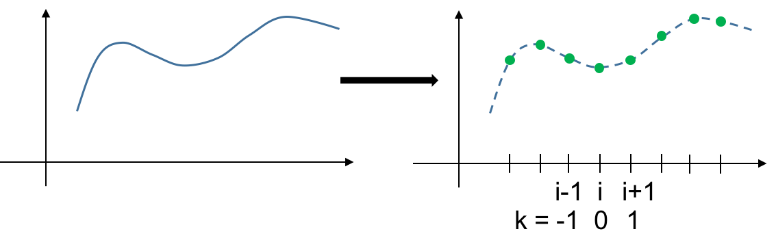
Get the derivative at $x_i$: $f^{\prime}(x_i)$, or call this $f^{\prime}_i$.
- Form Taylor series approximation to $f(x)$, centered on points about $i$.
- Combine these series to find derivatives at point $i$. Do the combinations in a way that gives desired cancellations.

Review Taylor Series

Given $f(x)$, express $f(x)$ as a power series: $$f(x) = a_0 + a_1x + a_2x^2 + a_3x^3+\ldots$$
Or, expand about $x_0$, which is equivalent: $$f(x) = c_0 + c_1(x-x_0) + c_2(x-x_0)^2 + c_3(x-x_0)^3+\ldots$$
Solve for the $c_i$. For $x=x_0$:
- $f(x_0) = c_0 \rightarrow c_0=f(x_0)$
- $f^{\prime}(x_0) = c_1 \rightarrow c_1 = f^{\prime}(x_0)$
- $f^{\prime\prime}(x_0) = 2c_2 \rightarrow c_2 = f^{\prime\prime}(x_0)/2$
- $f^{\prime\prime\prime}(x_0) = 3!c_3\rightarrow c_3 = f^{\prime\prime\prime}(x_0)/3!$
- etc.

$$f(x) = f(x_0) + f^{\prime}(x_0)(x-x_0) + \frac{1}{2}f^{\prime\prime}(x_0)(x-x_0)^2 + \frac{1}{3!}f^{\prime\prime\prime}(x_0)(x-x_0)^3+\ldots$$

$$ f(x) = \sum_{m=0}^n \frac{1}{m!}f^{(m)}(x_0)(x-x_0)^m + R_n(\xi),$$

$$ R_n(\xi) = \frac{1}{(n+1)!}f^{(n+1)}(\xi)(\xi-x_0)^{n+1},\,\,\, x\le\xi\le x_0.$$

Goal:

Get $f^{\prime}(x)$, or $f^{\prime\prime}(x)$, etc., from a Taylor Series.
- T.S. is written in terms of two or more points: $x_1$, $x_2$, etc.
- T.S. has multiple $f^{(n)}$, which we either don’t want, or don’t have.
- Truncate the T.S. $\rightarrow$ truncation error.
- Write T.S. for different points and combine each series to cancel undesired terms.
- The order of the truncation error term is the rate that the error approaches $0$ as $(x-x_0)\rightarrow 0.$
  - Order of the remainder term: $\mathcal{O}(\Delta x^n)$.

Example 1

Consider a grid with three points: $(i-1)---(i)---(i+1).$ $$f(x_{i+1}) = f(x_i) + f^{\prime}(x_i)(x_{i+1}-x_i) + \left[\frac{1}{2}f^{\prime\prime}(x_i)(x_{i+1}-x_i)^2+\ldots\right].$$

Solve for $f^{\prime}(x_i)$:

$$ f^{\prime}(x_i) = \frac{f(x_{i+1})-f(x_i)}{\Delta x} - \left[\frac{1}{2}f^{\prime\prime}\Delta x^2 / \Delta x+\ldots\right].$$ $$ f^{\prime}(x_i) = \frac{f(x_{i+1})-f(x_i)}{\Delta x} + \mathcal{O}(\Delta x).$$

This is a first order, forward difference approximation.
First order since the error term is $\mathcal{O}(\Delta x^1)$, that is $\Delta x$ to the power 1.
A backward difference version is also available if we consider points $i$ and $i-1$.

Example 2

Consider a grid with three points: $(i-1)---(i)---(i+1).$ $$f_{i+1} = f_i + f_i^{\prime}\Delta x + \frac{1}{2}f^{\prime\prime}_i\Delta x^2 + \frac{1}{6}f_i^{\prime\prime\prime}\Delta x^3 + \frac{1}{24}f^{\prime\prime\prime\prime}\Delta x^4 + \ldots,$$ $$f_{i-1} = f_i - f_i^{\prime}\Delta x + \frac{1}{2}f^{\prime\prime}_i\Delta x^2 - \frac{1}{6}f_i^{\prime\prime\prime}\Delta x^3 + \frac{1}{24}f^{\prime\prime\prime\prime}\Delta x^4 + \ldots,$$

Subtract the second equation from the first $\rightarrow$

$$ f_{i+1}-f_{i-1} = 2f_i^{\prime}\Delta x + \left[\frac{2}{6}f_i^{\prime\prime\prime}\Delta x^3+\ldots\right].$$

Solve for $f_i^{\prime}$:

$$f_i^{\prime} = \frac{f_{i+1}-f_{i-1}}{2\Delta x} - \left[\frac{1}{6}f_i^{\prime\prime\prime}\Delta x^3+\ldots\right]/\Delta x.$$

Or,

$$f_i^{\prime} = \frac{f_{i+1}-f_{i-1}}{2\Delta x} + \mathcal{O}(\Delta x^2).$$

This is a second order central difference approximation.
- Second order since the error term is $\mathcal{O}(\Delta x^2).$
- Higher order terms are neglected since they are considered small compared to this term.
- Notice that the symmetry cancelled the $\frac{1}{2}f_i^{\prime\prime}\Delta x^2$ terms $\rightarrow$ higher order, more accurate.

Example 3

Instead of subtracting the two equations of Example 2, add them instead:

$$f_{i+1}+f_{i-1} = 2f_i + \frac{2}{2}f_i^{\prime\prime}\Delta x^2 + \left[\frac{2}{24}f_i^{(iv)}\Delta x^4+\ldots\right].$$

Solve for $f_i^{\prime\prime}$

$$f_{i}^{\prime\prime} = \frac{f_{i-1}-2f_i+f_{i+1}}{\Delta x^2} - \mathcal{O}(\Delta x^2).$$

This is a second order central difference approximation of the second derivative.
When we add the two equations, the first derivative cancels.
This is commonly used for approximating terms like $\alpha\frac{d^2T}{dx^2}$ in diffusive problems, for example, in the heat conduction equation.
- Discretizing this equation on a grid results in a tridiagonal matrix.

Taylor Table

Generalize the finite difference (F.D.) approximations to any order derivative, to any order error.
Grid:

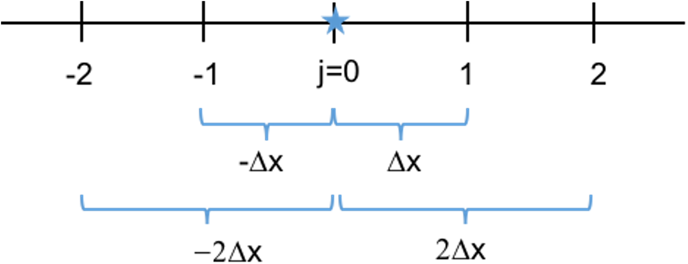
The F.D. approximation will be a linear combination of $f_j$ values
e.g.,

$$f_0^{\prime} = (c_{-2}f_{-2} + c_{-1}f_{-1} + c_0f_0 + c_1f_1 + c_2f_2]/\Delta x,$$

$$f_0^{\prime\prime} = (d_{-2}f_{-2} + d_{-1}f_{-1} + d_0f_0 + d_1f_1 + d_2f_2]/\Delta x^2.$$

$$\ldots$$

Taylor table

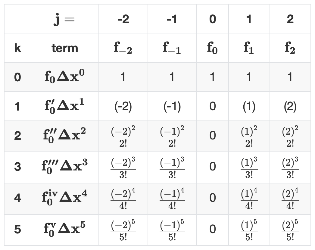
Column elements are coefficients of the T.S. terms on the left.
The sum of the first column (coefficients times terms) gives $f_{-2}$, and similar for other columns.

$$f_{-2} = (1)f_0 + (-2)f_0^{\prime}\Delta x + \frac{(-2)^2}{2!}f_0^{\prime\prime}\Delta x^2 + \frac{(-2)^3}{3!}f_0^{\prime\prime\prime}\Delta x^3 + \frac{(-2)^4}{4!}f_0^{iv}\Delta x^4 + \frac{(-2)^5}{5!}f_0^{v}\Delta x^5 \ldots.$$

For a term like $(-2)^2/2!$, the $(-2)^2$ is because we have $(-2\Delta x)^2 = (-2)^2\Delta x^2$ because we are $-2\Delta x$ away from $j=0$.
To take a linear combination, each column gets multiplied by some coefficient $c_j$ and we add these up.
- That is, we add the T.S. times $c_j$, for each point in the grid $\rightarrow$ linear combination of points.
We want the resulting coefficient of each term $f_0$, $f_0^{\prime}$, etc. to all be zero except the derivative we are approximating.
$\rightarrow$ the $\sum$ of each row, when we have columns times $c_j$ are 0, except the desired derivative, which is $1$.
Form a linear system: $Ac=b$ where $c$ are the coefficients of the linear combinations, $b^{T} = [0,1,0,0,0,0]$ for a first derivative, or $b^T = [0,0,1,0,0,0]$ for a second derivative, etc. The elements of $A$ are in the table above:
$$A_{kj} = j^{k}/k!$$
Order of the error is $k-(\mbox{order of derivative})$, where $k$ is the first row with a nonzero sum.

Example

For an $\mathcal{O}(\Delta x^2)$ approximation to $f^{\prime}$ $$\left[ \begin{array}{ccc} 1 & 1 & 1 \\ -1 & 0 & 1 \\ \frac{1}{2} & 0 & \frac{1}{2} \\ \end{array} \right] \left[ \begin{array}{c} c_{-1} \\ c_0 \\ c_1 \end{array} \right] = \left[ \begin{array}{c} 0 \\ 1 \\ 0 \end{array} \right] $$

$$\rightarrow c = \left[ \begin{array}{c} -\frac{1}{2} \\ 0 \\ \frac{1}{2} \end{array} \right] $$

This gives

$$f_0^{\prime}\approx\frac{1}{\Delta x}\left[-\frac{1}{2}f_{-1} + 0f_0 + \frac{1}{2}f_1\right] = \frac{f_1 - f_{-1}}{2\Delta x}.$$

* Here, we have a 3 point stencil, where the base point is 2 of 1, 2, or 3 (the middle). * Order: $\vec{R}_3^T\cdot\vec{c} = 1/6 \ne 0\rightarrow k=3 \rightarrow$ order = 3-1 = 2$^{nd}$ order approximation. * That is row 3 dotted with vector c = $1/6\ne0$. * $[-1/6,\, 0,\, 1/6]\cdot [-1/2,\,0,\,1/2] = 1/6$.

Example

For a 1-sided $\mathcal{O}(\Delta x^2)$ approximation to $f^{\prime}$
Take $j=0,\,1,\,2$ of the table.
- Three point stencil, with base point 1 of 1, 2, or 3.

$$\left[ \begin{array}{ccc} 1 & 1 & 1 \\ 0 & 1 & 2 \\ 0 & \frac{1}{2} & 2 \\ \end{array} \right] \left[ \begin{array}{c} c_{-1} \\ c_0 \\ c_1 \end{array} \right] = \left[ \begin{array}{c} 0 \\ 1 \\ 0 \end{array} \right] $$$$\rightarrow c = \left[ \begin{array}{c} -\frac{3}{2} \\ 2 \\ -\frac{1}{2} \end{array} \right] $$

This gives

$$f_0^{\prime}\approx\frac{1}{\Delta x}\left[-\frac{3}{2}f_0 + 2f_1 - \frac{1}{2}f_2\right] $$

$\vec{R}_3^T\cdot \vec{c} = -1/3\ne 0$.
- So, the order is $k-1 = 3-1 = 2$ or 2$^{nd}$ order.
- $[0,\,1/6,\,4/3]\cdot[-3/2,\,2,\,-1/2] = -1/3$.

Taylor table code

Finite difference approximations to arbitrary order derivatives, using arbitrary stencils.

$$\frac{d^n u}{dx^n} = \frac{1}{\Delta x^n}\sum_k c_ku_k$$

As an example, a second order central second difference:

$$\frac{d^2 u}{dx^2} = \frac{1}{\Delta x^2}(c_{j-1} + c_ju_j + c_{j+1}u_{j+1}),$$

with $c$’s are 1, -2, 1
We assume here that $j=0$ is the base point.

import numpy as np

#----------------------

oDer = 1     # order of the derivative to approximate (like 1 for f', or 2 for f", etc.)
npts = 9     # number of points in the stencil. Min is oDer + 1.
jb   = 5     # position of the base point in the stencil, starting at 1
             # the setup: oDer=1, npts=3, jb=2, will give a second order central difference approx to f'

#----------------------

jp = np.arange(1-jb, npts-jb+1)   # index in grid: like [-2 -1 0 1 2 ] for jp=3 for npts=5
a_kj = np.zeros((npts,npts))
    
j = np.arange(npts)
for k in range(npts) :
    a_kj[k,j] = jp[j]**k / np.math.factorial(k)
b = np.zeros(npts)
b[oDer] = 1
c_u = np.linalg.solve(a_kj,b)
                             #  check the order
aa = np.zeros(npts)
for k in range(oDer+1,100) :           
    aa[j] = (jp[j]**k)/np.math.factorial(k)
    if np.abs(np.sum(aa*c_u)) > 1.0E-10 :
        break
        
#----------------------
                            # output the results
print('Grid_position (top), coefficient (bottom) =\n')
print(np.vstack([jp, c_u]))
print('\nOrder = ', k-oDer)

Grid_position (top), coefficient (bottom) =

[[-4.00000000e+00 -3.00000000e+00 -2.00000000e+00 -1.00000000e+00
   0.00000000e+00  1.00000000e+00  2.00000000e+00  3.00000000e+00
   4.00000000e+00]
 [ 3.57142857e-03 -3.80952381e-02  2.00000000e-01 -8.00000000e-01
  -4.91828800e-15  8.00000000e-01 -2.00000000e-01  3.80952381e-02
  -3.57142857e-03]]

Order =  8

/var/folders/xr/cv4msgs94jq0nw15cwkskrbc0000gn/T/ipykernel_28096/850803756.py:17: DeprecationWarning: `np.math` is a deprecated alias for the standard library `math` module (Deprecated Numpy 1.25). Replace usages of `np.math` with `math`
  a_kj[k,j] = jp[j]**k / np.math.factorial(k)
/var/folders/xr/cv4msgs94jq0nw15cwkskrbc0000gn/T/ipykernel_28096/850803756.py:24: DeprecationWarning: `np.math` is a deprecated alias for the standard library `math` module (Deprecated Numpy 1.25). Replace usages of `np.math` with `math`
  aa[j] = (jp[j]**k)/np.math.factorial(k)

import sympy as sp
sp.init_printing(long_frac_ratio=1)
import numpy as np
from sympy.printing.latex import LatexPrinter
from IPython.display import Markdown as md                         # hack to pretty output the latex...

#----------------------

oDer = 1     # order of the derivative to approximate (like 1 for f', or 2 for f", etc.)
npts = 9     # number of points in the stencil. Min is oDer + 1.
jb   = 5     # position of the base point in the stencil, starting at 1
             # the setup: oDer=1, npts=3, jb=2, will give a second order central difference approx to f'

#----------------------

jp = np.arange(1-jb, npts-jb+1, dtype=np.int32)   # index in grid: like [-2 -1 0 1 2 ] for jp=3 for npts=5

A = sp.zeros(npts,npts)
for k in range(npts):
    for j in range(npts):
        A[k,j] = jp[j]**k / sp.factorial(k)
B = sp.zeros(npts,1)
B[oDer] = 1
C = A**-1 * B
c = np.array(C.T).astype(np.float64)[0]           # numpy array of coefficients

#---------------------- check the order
j = np.arange(npts)
for k in range(oDer+1,100) :           
    aa = (jp[j]**k)/np.math.factorial(k)
    if np.abs(np.sum(aa*c)) > 1.0E-10 :
        break
        
#---------------------- output results

points = [sp.symbols(f'u_{j}') for j in jp]
Δx, u, x, = sp.symbols('Δx, u, x')
u0 = sp.symbols('u_0')

rr = []
for i in range(npts):
    rr.append(C[i]*points[i])
rhs = sp.Add(*rr,evaluate=False) # keep the order of the additive terms...

lhs = LatexPrinter(dict(order='none'))._print(sp.Derivative(u0,x,oDer))
rhs = LatexPrinter(dict(order='none'))._print_Add(rhs)
expr = lhs + "=" + rhs + f"+O(\Delta x^{k-oDer})"

md(f"$${expr}$$")

<>:47: SyntaxWarning: invalid escape sequence '\D'
<>:47: SyntaxWarning: invalid escape sequence '\D'
/var/folders/xr/cv4msgs94jq0nw15cwkskrbc0000gn/T/ipykernel_28096/2778617435.py:47: SyntaxWarning: invalid escape sequence '\D'
  expr = lhs + "=" + rhs + f"+O(\Delta x^{k-oDer})"
/var/folders/xr/cv4msgs94jq0nw15cwkskrbc0000gn/T/ipykernel_28096/2778617435.py:30: DeprecationWarning: `np.math` is a deprecated alias for the standard library `math` module (Deprecated Numpy 1.25). Replace usages of `np.math` with `math`
  aa = (jp[j]**k)/np.math.factorial(k)

$$\frac{d}{d x} u_{0}=\frac{u_{-4}}{280} - \frac{4 u_{-3}}{105} + \frac{u_{-2}}{5} - \frac{4 u_{-1}}{5} + 0 + \frac{4 u_{1}}{5} - \frac{u_{2}}{5} + \frac{4 u_{3}}{105} - \frac{u_{4}}{280}+O(\Delta x^8)$$

$\displaystyle \left[\begin{matrix}\frac{1}{280}\\\\- \frac{4}{105}\\\\ \frac{1}{5}\\\\- \frac{4}{5}\\\\0\\\\ \frac{4}{5}\\\\- \frac{1}{5}\\\\ \frac{4}{105}\\\\- \frac{1}{280}\end{matrix}\right]$