ChEn 433 Thermodynamics
Class 5
Carnot Process
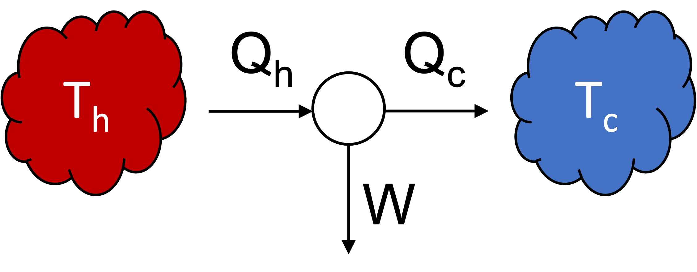

- Isothermal heat transfer: hot reservoir to working fluid at \(T_h\).
- Adiabatic expansion of working fluid to \(T_c\).
- Isothermal heat transfer: working fluid to cold reservoir at \(T_c\).
- Adiabatic compression of working fluid to \(T_h\).
label the figure with heat and work flows
Carnot Efficiency
\[W = Q_h - Q_c =
Q_h\left(1-\frac{Q_c}{Q_h}\right)\] \[Q_c = T_cΔS_c,\,\,\,\,\, Q_h = -T_hΔS_h\]
\[W = Q_h\left(1-\frac{T_cΔ S_c}{-T_hΔ
S_h}\right)\] For a reversible process, \(Δ S_c = -Δ S_h\), so
\[W = Q_h\left(1-\frac{T_c}{T_h}\right),\,\,\,η=\left(1-\frac{T_c}{T_h}\right)\]
Work from Heat Transfer: simple configuration
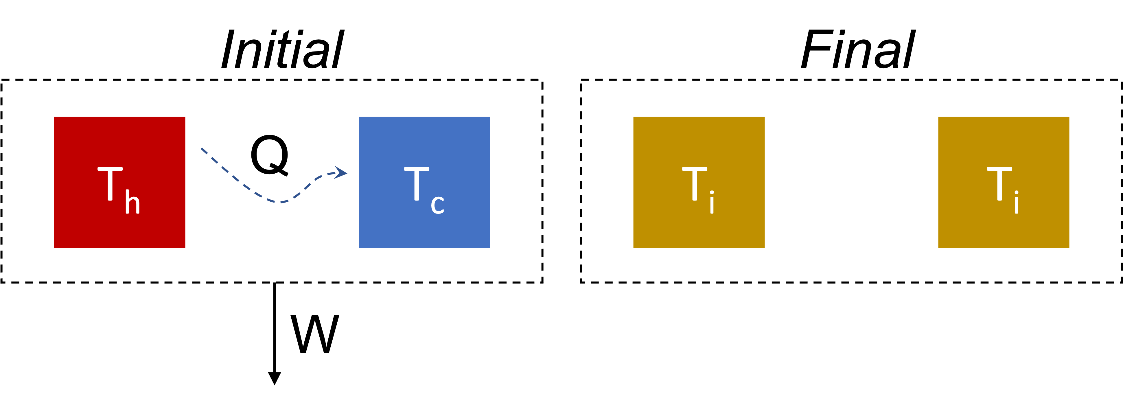
- Consider heat transfer between two objects.
- The two objects constitute the system.
- objects have constant and equal heat capacities \(C\),
- fixed volumes.
- Heat is exchanged and work is extracted from the system.
- Find the maximum work.
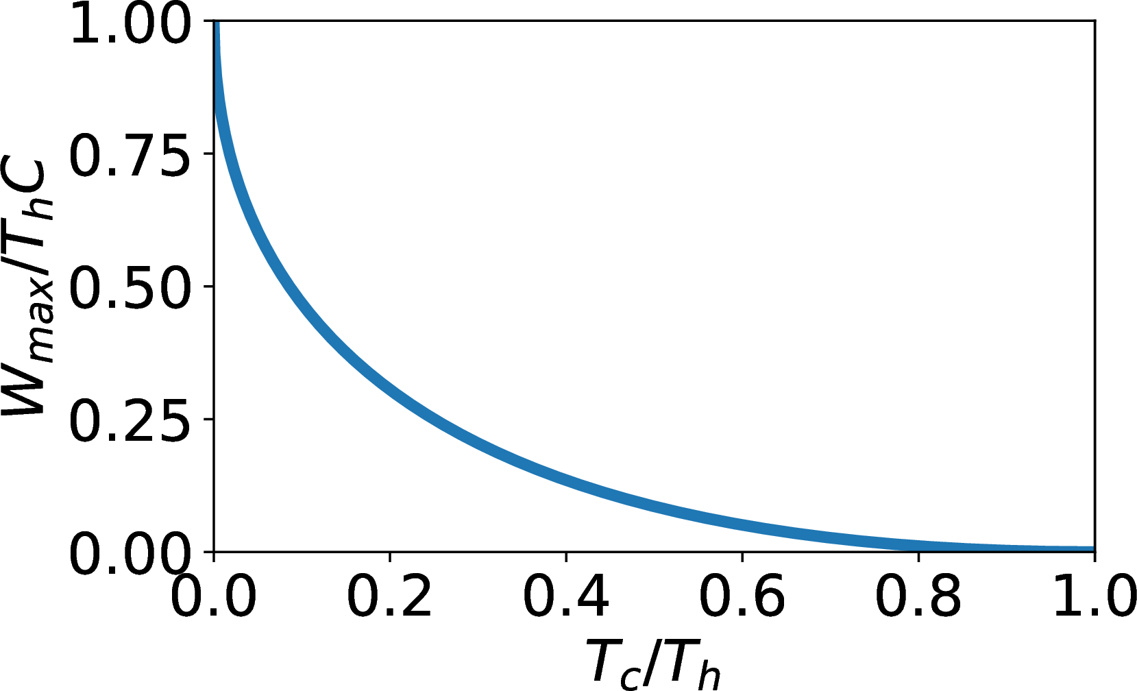
Work from Heat Transfer: efficiency
- \((W_{max}/C)_{max}=T_h\) at \(T_c=0\).
- \((W_{max}/C)_{min}=0\) at \(T_c=T_h\).
- Efficiency
- take the hot object as the driver
- normalize the work by \(Δ U_h\)
\[\begin{align}
η &= \frac{W/C}{Δ U_h/C}, \\
η &= \frac{T_h + T_c -
2\sqrt{T_hT_c}}{T_h-\underbrace{\sqrt{T_hT_c}}_{T_i}} =
1-\sqrt{\frac{T_c}{T_h}}.
\end{align}\]
\[η = 1-\sqrt{\frac{T_c}{T_h}}.\]
Work from Heat Transfer: plot
Parameterize \(T_{h2}\), which varies from \(T_h\) to \(\sqrt{T_cT_h}\), using progress variable \(ξ\): \[T_{h2} = T_h(1-ξ) + \sqrt{T_cT_h}(ξ)\] Insert into the expression for \(η\) \[η = \frac{r + ξ(1-\sqrt{r}) - \frac{r}{1-ξ+ξ\sqrt{r}}}{ξ(1-\sqrt{r})},\] where \(r = T_c/T_h\).
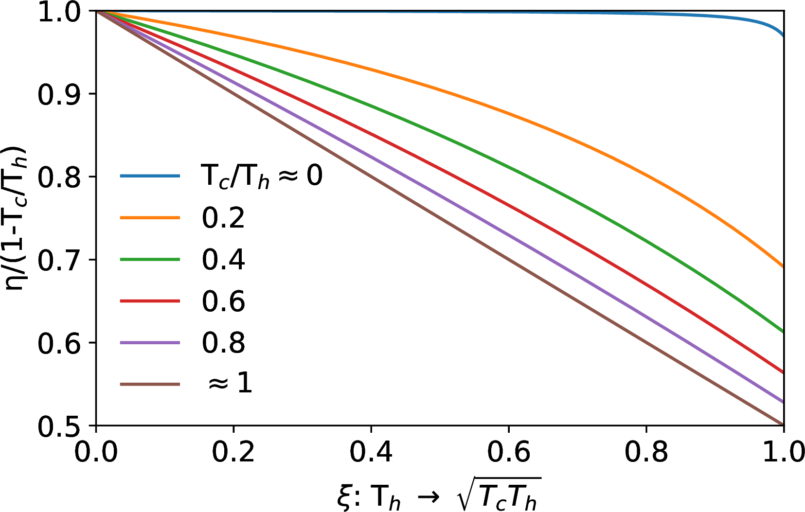 The Carnot
efficiency is achieved when heat transfer occurs to and from infinite
reservoirs, whose temperature does not change during the heat
transfer.
The Carnot
efficiency is achieved when heat transfer occurs to and from infinite
reservoirs, whose temperature does not change during the heat
transfer.
Or, between finite objects, when very little heat transfer is allowed to occur, so that the object temperatures effectively don’t change.